Manufacturing Maintenance Case Study

Say we have a large amount of historical maintenance work-order (MWO) data stored up, but we don’t quite know what to do with it yet. This case study will walk through the initial parsing of the MWO natural-language data from the technicians, to some preliminary analysis of machines, and finally visualization of potential failure modes maintenance request types. Hopefully it will give you a good idea of how Nestor can assist you in analyzing the rich, existing data in your MWO’s, and how easy it can be to correlate it to other fields you might be recording.

The primary workflow for Nestor in this case study (when used as a python library) is:

1. Import data, determining

   • what columns contain useful (well-defined) categories

   • what columns contain natural language to be tagged with the Nestor UI

   • what columns could be used for date-stamping/time-series analysis

2. Perform any cleaning necessary on categorical and time-series data.

   • This is not necessarily within the scope of Nestor, but:

   • Python+Pandas makes it fairly straight forward

   • and compatible with the Nestor output tags!

3. Tag natural language data using Nestor/NestorUI

   • Nestor can give you initial statistics about your data, immediately, but:

   • Nestor is built as a human-in-the-loop tool, meaning that

   • you will be a crucial part of the process, and Nestor makes implementing your annotation lightning-fast.

4. Import the tags created by Nestor, and perform analyses

   • Nestor UI is designed to create a vocabulary file, quickly mapping discovered concepts to clean tags.

   • we’ve also built several tools to help you perform initial analyses on the tags (with more to come!)

We’ll start by loading up some common packages and setting our plotting style (for consistency):

from pathlib import Path
import numpy as np
import pandas as pd
import seaborn as sns
import matplotlib.pyplot as plt
%matplotlib inline

/home/tbsexton/anaconda3/lib/python3.6/importlib/_bootstrap.py:219: RuntimeWarning: numpy.dtype size changed, may indicate binary incompatibility. Expected 96, got 88
  return f(*args, **kwds)
/home/tbsexton/anaconda3/lib/python3.6/importlib/_bootstrap.py:219: RuntimeWarning: numpy.dtype size changed, may indicate binary incompatibility. Expected 96, got 88
  return f(*args, **kwds)

def set_style():
    # This sets reasonable defaults for font size for a figure that will go in a paper
    sns.set_context("paper")
    # Set the font to be serif, rather than sans
    sns.set(font='serif')
    # Make the background white, and specify the specific font family
    sns.set_style("white", {
        "font.family": "serif",
        "font.serif": ["Times", "Palatino", "serif"]
    })
set_style()

For the interactive plots we’ll need Holoviews, with the Bokeh backend:

Data Preparation

Import Data

Nestor will be parsing through the NLP data soon, but first we need to determine what else might be useful for us. In this case study, we’ll be using the recorded machine number, the date the MWO was recieved, technician names, and of course, the written descriptions left by our technicians.

In this particular case, we’ll be focusing primarily on the (anonymized) machine types A and B.

data_dir = Path('../..')/'data'/'sme_data'
df = pd.read_csv(data_dir/'MWOs_anon.csv')

df.date_received = pd.to_datetime(df.date_received)
print(f'There are {df.shape[0]} MWO\'s in this dataset')

There are 3438 MWO's in this dataset

# example data:
df.loc[df.mach.str.contains('A\d|B\d', na=False),
       ['mach', 'date_received', 'issue', 'info', 'tech']].head(10)

	mach	date_received	issue	info	tech
0	A5	2015-01-14	No power	Replaced pin in pendant and powered machine -P...	angie_henderson, michele_williams
2	A18	2015-02-27	Check / Charge Accumulators	Where OK	nathan_maldonado
3	A23	2015-02-27	Hyd leak at saw atachment	Replaced seal in saw attachment but still leak...	michele_williams
4	A24	2015-02-27	CS1008 setup change over / from ARC1004	Completed / Threading unit rewired	ethan_adams, michele_williams
5	A27	2015-02-27	Gears on saw attachment tight and grinding per...	Replaced saw attachment with rebuilt unit / Re...	michele_williams
6	A33	2015-02-27	Check and charge Accumulators	Checked and charged	cristian_santos
7	A8	2015-02-27	St# 14 milling spindle repairs	Reapired	michele_williams
8	B2	2015-02-27	Hydraulic leak	Replaced ruptured hydraulic line Side B	gina_moore, dylan_miller
9	B3	2015-02-27	Turrets leaking A & B	Turrets removed and cleaned of chhips	nathan_maldonado
10	B5	2015-02-27	Spindle carrier not indexing / Over Feed	NaN	gina_moore, dylan_miller

Starting Nestor

The first thing we can do is collect, combine, and cleanse our NLP data, to get a better idea of what it looks like going into Nestor. To do this, let’s import the main text mining module in Nestor, nestor.keyword, which helps us with keyword definition and extraction.

The NLPSelect object is a transformer in the style of scikit-learn, which will take in defined names for columns containing our original NLP data, and transform that data with it’s .transform() method.

from nestor import keyword as kex
# merge and cleanse NLP-containing columns of the data
nlp_select = kex.NLPSelect(columns = ['issue', 'info'])
raw_text = nlp_select.transform(df)

/home/tbsexton/anaconda3/lib/python3.6/importlib/_bootstrap.py:219: RuntimeWarning: numpy.dtype size changed, may indicate binary incompatibility. Expected 96, got 88
  return f(*args, **kwds)
/home/tbsexton/anaconda3/lib/python3.6/importlib/_bootstrap.py:219: RuntimeWarning: numpy.dtype size changed, may indicate binary incompatibility. Expected 96, got 88
  return f(*args, **kwds)

Let’s see what the most common MWO’s in our data look like, without the punctuation or filler-words to get in the way:

raw_text.value_counts()[:10]

base cleaning requested completed                 15
broken bar feeder chain repaired                  14
base needs to be cleaned completed                 7
broken feeder chain repaired                       5
chip conveyor jam cleared                          5
bar feeder chain broken repaired                   5
bar loader chain broken repaired                   5
base clean completed                               3
replace leaking dresser control valve replaced     3
workzone light inop                                3
dtype: int64

Interesting. We see a number of repetitive base-cleaning requests being entered in identically, along with some requests to fix a broken chain on the bar-feeder. However, there’s alarmingly verbatim repeats, and we see a lot of overlap even in the top 10 there. This is where Nestor comes in.

Similar to the above, we can make a TokenExtractor object that will perform statistical analysis on our corpus of MWO’s, and return the concepts it deems “most important”. There’s a lot in here, but essentially we will get an output of the most important concepts (as tokens) in our data. We do this with the scikit-learn TfIdfVectorizer tool (which transforms our text into a bag-of-words vector model), along with some added features, like a method to score and rank individual concepts.

Let’s see what tokens/concepts are most important:

tex = kex.TokenExtractor()
toks = tex.fit_transform(raw_text)  # bag of words matrix.

print('Token\t\tScore')
for i in range(10):
    print(f'{tex.vocab_[i]:<8}\t{tex.scores_[i]:.2e}')

Token           Score
replaced        1.86e-02
broken          9.68e-03
st              9.51e-03
unit            8.41e-03
inop            7.27e-03
motor           7.21e-03
spindle         7.17e-03
leak            6.88e-03
repaired        6.75e-03
valve           6.74e-03

These are small scores, but they’re normalized to add to 1:

tex.scores_.sum()

1.0

Note that the current default is to limit the number of extracted concepts to the top 5000 (can be modified in the TokenExtractor kwargs, but in practice should be more than sufficient.

Nestor UI and Tags

vocab_fname = data_dir/'vocab.csv'
vocab = kex.generate_vocabulary_df(tex, filename=vocab_fname)
tags_df = kex.tag_extractor(tex, raw_text, vocab_df=vocab)

attempting to initialize with pre-existing vocab
intialized successfully!
saved locally!
intialized successfully!

tags_read = kex._get_readable_tag_df(tags_df)
tags_read.join(df[['issue', 'info', 'tech']]).head(4)

	I	NA	P	S	U	X	issue	info	tech
0	machine, cable, pin, pendant	possible, powered	short	replaced	power		No power	Replaced pin in pendant and powered machine -P...	angie_henderson, michele_williams
1	part	repaired, tech, harness, smartscope	broken	order			Smartscope harness broken	Parts ordered / Tech repaired	gina_moore, tech
2	accumulator			check, charge, ok			Check / Charge Accumulators	Where OK	nathan_maldonado
3	hydraulic, saw, attachment, marcel_l	reapirs, pending	leak	replaced	seal		Hyd leak at saw atachment	Replaced seal in saw attachment but still leak...	michele_williams

# how many instances of each keyword class are there?
print('named entities: ')
print('I\tItem\nP\tProblem\nS\tSolution\nR\tRedundant')
print('U\tUnknown\nX\tStop Word')
print('tagged tokens: ', vocab[vocab.NE!=''].NE.notna().sum())
print('total tags: ', vocab.groupby("NE").nunique().alias.sum())
vocab.groupby("NE").nunique()

named entities:
I       Item
P       Problem
S       Solution
R       Redundant
U       Unknown
X       Stop Word
tagged tokens:  518
total tags:  294

	NE	alias	notes	score
NE
	1	2	1	2485
I	1	149	8	280
P	1	26	1	63
S	1	27	1	57
U	1	86	6	113
X	1	4	1	4

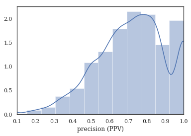
# tag-completeness of work-orders?
tag_pct, tag_comp, tag_empt = kex.get_tag_completeness(tags_df)

nbins = int(np.percentile(tags_df.sum(axis=1), 90))
print(f'Docs have at most {nbins} tokens (90th percentile)')

sns.distplot(tag_pct.dropna(), bins=nbins, kde_kws={'cut':0})
plt.xlim(0.1, 1.0)
plt.xlabel('precision (PPV)')

Tag completeness: 0.72 +/- 0.19
Complete Docs: 514, or 14.95%
Empty Docs: 20, or 0.58%
Docs have at most 13 tokens (90th percentile)

/home/tbsexton/anaconda3/lib/python3.6/site-packages/scipy/stats/stats.py:1713: FutureWarning: Using a non-tuple sequence for multidimensional indexing is deprecated; use `arr[tuple(seq)]` instead of `arr[seq]`. In the future this will be interpreted as an array index, `arr[np.array(seq)]`, which will result either in an error or a different result.
  return np.add.reduce(sorted[indexer] * weights, axis=axis) / sumval

Text(0.5,0,'precision (PPV)')

Context Expansion (simplified)

Nestor now has a convenience function for generating 1- and 2-gram tokens, and extracting “good” tags from your MWO’s once given the 1- and 2-gram vocabulary files generated by the nestor-gui application. This makes our life easier, though the functionality is planned to be deprecated and replaced by a more robust pipelining tool fashined after the Scikit-Learn Pipeline model.

vocab = pd.read_csv(vocab_fname, index_col=0)
vocab2 = pd.read_csv(data_dir/'2g_vocab.csv', index_col=0)

tag_df, tag_relation, NA_df = kex.ngram_keyword_pipe(raw_text, vocab, vocab2)

calculating the extracted tags and statistics...

 ONE GRAMS...
intialized successfully!

found bug!       None

 TWO GRAMS...
intialized successfully!

We can also get a version of the tags that is human-readable, much like the tool in nestor-gui. Though less useful for plotting/data-analysis, this is great for a sanity check, or for users that prefer visual tools like Excel.

all_tags = pd.concat([tag_df, tag_relation])
tags_read = kex._get_readable_tag_df(all_tags)
tags_read.head(10)

	I	P	P I	S	S I	U
0	cable, machine, pendant, pin	short		replaced		power
1	part	broken		order
2	accumulator			charge, check, ok
3	attachment, hydraulic, marcel_l, saw, saw atta...	leak		replaced		seal
4	thread, thread unit, unit			setup		change
5	alex_b, attachment, gear, saw, saw attachment,...			rebuild, remove, replaced
6	accumulator			charge, check
7	mill, spindle, station			repair		14
8	hydraulic, hydraulic line, line	leak, rupture		replaced
9	turret	leak		clean, remove

Measuring Machine Performance

The first thing we might want to do is determine which assets are problematic. Nestor outputs tags, which need to be matched to other “things of interest,” whether that’s technicians, assets, time-stamps, etc. Obviously not every dataset will have every type of data, so not all of these analyses will be possible in every case (a good overview of what key performance indicators are possible with what data-type can be found here).

Since we have dates and assets associated with each MWO, let’s try to estimate the failure inter-arrival times for machines by type and ID.

Failure Inter-arrival Times, by Machine

Ordered by total occurences (i.e. “distribution certainty”)

• Time between occurences of broken tag.

• low \(\rightarrow\) bad

• e.g. A34, B19, and A14 all seem rather low

What could be the central problems with these machines? While we’re at it, let’s use the wonderful library Lifelines to calculate the Survival functions of our different machine types. We can again use tags to approximate relevant data we otherwise would not have had: censoring of observations is not obvious, but we can guess that replacements (without broken) generally indicate a machine was swapped before full breakdown/end-of-life.

import warnings
warnings.simplefilter(action='ignore')

# make sure Pandas knows our column is a proper Datetime.
idx_col = pd.DatetimeIndex(df.date_received)

# match the A and B machines, checking if they were "broken"
h_or_i = (df
    .mach
    .str
    .match(r'^[AB][0-9]*$')
    .fillna(False)
)
is_broke = (tag_df.P['broken']>0)
cond = h_or_i & is_broke
sample_tag = tag_df.loc[cond,tag_df.loc[cond].sum()>1]
sample_tag.columns = (sample_tag
    .columns
    .droplevel(0)
)

# Add tags back to original data
sample_tag = pd.concat([sample_tag, df.mach[cond]], axis=1)
sample_tag['date'] = idx_col[cond]
sample_tag.loc[:,'mach_type'] = sample_tag.mach.str[0]

# Time between failure, BY MACHINE, for entire dataset.
sample_tag['tbf'] = (sample_tag
    .sort_values(['mach','date'])
    .groupby('mach')['date']
    .diff()
)
sample_tag.loc[:,'tbf'] = sample_tag.tbf/pd.Timedelta(days=1)  # normalize time to days

# keep relevant data
samps = sample_tag[['mach_type', 'tbf', 'mach']].dropna()
order = (samps
    .mach
    .value_counts()
    .index
)  # from most to least no. of examples

# Box-and-whisker plot for TBF
import matplotlib.gridspec as gridspec
# plt.figure(figsize=(5,10))
fig = plt.figure(tight_layout=True, figsize=(12,8))
gs = gridspec.GridSpec(2, 2)
ax1 = fig.add_subplot(gs[:,0])
sns.boxplot(data=samps, y='mach', x='tbf',
            hue='mach_type', orient='h',
            order=order[:20], notch=False,
           ax = ax1)
plt.xlabel('days');
plt.title('Time Between Failure ("broken")')
ax1.set(xlim=(0,250));
sns.despine(ax=ax1, left=True, trim=True)


#### Lifelines Survival Analysis ####
from lifelines import WeibullFitter, ExponentialFitter, KaplanMeierFitter

def mask_to_ETraw(df_clean, mask, fill_null=1.):
    """Need to make Events and Times for lifelines model
    """
    filter_df = df_clean.loc[mask]
    g = filter_df.sort_values('date_received').groupby('mach')
    T = g['date_received'].transform(pd.Series.diff)/pd.Timedelta(days=1)

    # assume censored when parts replaced (changeout)
    E = (~(tag_df.S['replaced']>0)).astype(int)[mask]
    T_defined = (T>0.)&T.notna()
    return T[T_defined], E[T_defined]

ax3 = fig.add_subplot(gs[-1,-1])
ax2 = fig.add_subplot(gs[0,-1], sharex=ax3)

T, E = mask_to_ETraw(df, cond)
kmf = KaplanMeierFitter()
kmf.fit(T, event_observed=E, label='Machine K-M')
kmf.plot(show_censors=True, censor_styles={'marker':'|'}, ax=ax2, color='xkcd:gray')
ax2.set(xlim=(0,250), ylabel=r'$S(t)$', title='Kaplan-Meier Survival Function');
sns.despine(ax=ax2, bottom=True, trim=True)

i_ = df.mach.str.match(r'^[B][0-9]*$').fillna(False)
T, E = mask_to_ETraw(df, i_&is_broke)
kmf.fit(T, event_observed=E, label='B-type K-M')
kmf.plot(show_censors=True, censor_styles={'marker':'|'}, ax=ax3)

h_ = df.mach.str.match(r'^[A][0-9]*$').fillna(False)
T, E = mask_to_ETraw(df, h_&is_broke)
kmf.fit(T, event_observed=E, label='A-type K-M')
kmf.plot(show_censors=True, censor_styles={'marker':'|'}, ax=ax3)


ax3.set(xlim=(0,250), ylabel=r'$S(t)$', xlabel='days');
sns.despine(ax=ax3,  trim=True)

<Figure size 360x720 with 0 Axes>

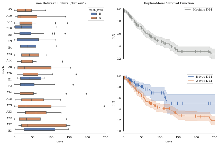
Markers ( | ) indicate a censored observation, interpreted as a maintenance event with no replacements (no ‘replaced’ tag occurrence).

• where “problems” aren’t listed, issue is generally routine maintenance.

• Assumption: Problem and Solution tags are almost entirely independent sets.

• We get a precise list of what isn’t known for free…the “Unknowns”.

Top Tag occurences, by Machine

Now that we’ve narrowed our focus, we can start to figure out 1. what is happening most often for each machine 2. what things are correlated when the happen 3. what the “flow” of diagnosis–>solution is for the machines.

from nestor.tagplots import color_opts
machs = ['A34', 'B19', 'A14']
def machine_tags(name, n_reps):
    ismach = df['mach'].str.contains(name, case =False).fillna(False)
    return tag_df.loc[ismach,(tag_df.loc[ismach,:].sum()>=n_reps).values]
f, ax = plt.subplots(ncols=3, figsize=(15, 5))

for n, mach in enumerate(machs):
    mach_df = machine_tags(mach,  6).sum().sort_values()
    mach_df.plot(kind='barh', color=[color_opts[i] for i in mach_df.index.get_level_values(0)], ax=ax[n])
    ax[n].set_title(mach)
    sns.despine(ax=ax[n], left=True)
plt.tight_layout()

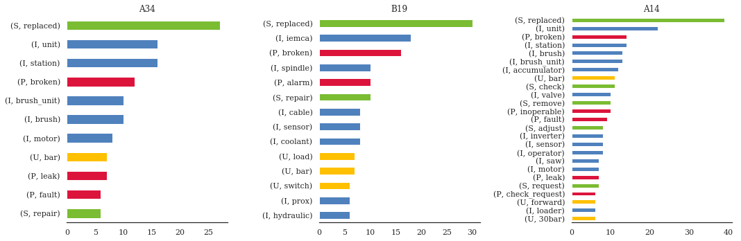
• A34 issues with motor, unit, brush

• B19 alarms and/or sensors, potentially coolant-related

• A14 wide array of issues, including operator (!?)

import holoviews as hv
hv.extension('bokeh')
%opts Graph [width=600 height=400]

%%output size=150 backend='bokeh' filename='machs'
%%opts Graph (edge_line_width=1.5, edge_alpha=.3)
%%opts Overlay [width=400 legend_position='top_right' show_legend=True] Layout [tabs=True]
from nestor.tagplots import tag_relation_net
import networkx as nx
kws = {
    'pct_thres':50,
    'similarity':'cosine',
    'layout_kws':{'prog':'neatopusher'},
    'padding':dict(x=(-1.05, 1.05), y=(-1.05, 1.05)),
      }

layout = hv.Layout([tag_relation_net(machine_tags("A34",  2), name='A34',**kws),
                    tag_relation_net(machine_tags("B19",  2), name='B19',**kws),
                    tag_relation_net(machine_tags("A14",  2), name='A14',**kws)
                   ])
layout

Measuring Technician Performance

is_base_cleaner = df.tech.str.contains('margaret_hawkins_dds').fillna(False)
print('Margaret\'s Top MWO\'s')
df['issue'][is_base_cleaner].value_counts()

Margaret's Top MWO's

Base cleaning requested                                              14
Base needs to be cleaned                                              8
Clean base                                                            4
Base clean                                                            3
Base cleaning req                                                     2
Cooling unit faults                                                   2
Base required cleaning                                                2
Base cleaning                                                         2
Base cleaning -caused fire                                            1
Chips in base obstructin coolant flow to pump                         1
Shipping cart has worn wheels                                         1
Base clean request before setup                                       1
Repair paper filter system                                            1
Base cleaning Requested                                               1
Base full                                                             1
Base needs to be cleaned -Opers overfilling and spilling on floor     1
Clean base to install SS chip catcher                                 1
Parts receiver prox cable shorting sensor                             1
Clean base -coolant sticky                                            1
Hydraulic contamination                                               1
Drain and clean tank -Do not refill                                   1
Base cleaning                                                         1
Base cleaning requested -Oil lines clogging                           1
Coolant tank needs to be cleaned                                      1
Clean out Sinico                                                      1
Base has hydraulic fluid -Drain/Clean                                 1
Coolant base needs to be cleaned                                      1
Base and coolant tank cleaning requested                              1
Oil site glass leaking on to floor                                    1
Name: issue, dtype: int64

# df['Description'][df['Tech Full Name'].str.contains('Lyle Cookson').fillna(False)]

def person_tags(name, n_reps):
#     techs = kex.token_to_alias(kex.NLPSelect().transform(df.tech.to_frame()), tech_dict)
    isguy = df.tech.str.contains(name).fillna(False)

    return tag_df.loc[isguy,(tag_df.loc[isguy,:].sum()>=n_reps).values]

people = ['margaret_hawkins_dds',
          'nathan_maldonado',
          'angie_henderson',
         ]
marg_df = person_tags(people[0],  5).sum().sort_values()

plt.figure(figsize=(5,5))
marg_df.plot(kind='barh', color=[color_opts[i] for i in marg_df.index.get_level_values(0)])
sns.despine(left=True)
plt.title('Margaret');

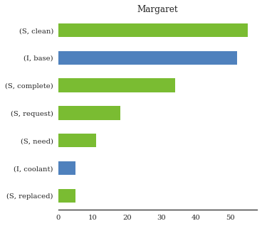
Threshold to tags happening >=5x - we can quickly gauge the number of Margaret’s total “base cleanings” as 45-50 - Say we want to compare with other, more “typical” technicians…

\(\rightarrow\) small problem…

f, ax = plt.subplots(ncols=3, figsize=(15, 5))
thres = [5, 20, 20]
for n, mach in enumerate(people):
    mach_df = person_tags(mach,  thres[n]).sum().sort_values()
#         mach_df = mach_df[mach_df>=5]
    mach_df.plot(kind='barh', color=[color_opts[i] for i in mach_df.index.get_level_values(0)], ax=ax[n])
    ax[n].set_title(mach.split(' ')[0])
    sns.despine(ax=ax[n], left=True)
plt.tight_layout()

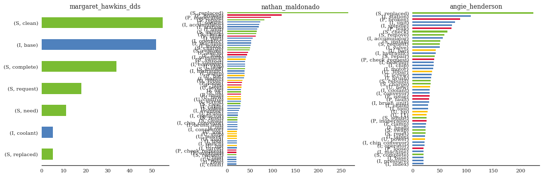
That’s very difficult to read. We could go back to our node-link, but because there is some directionality in how the technician addresses an MWO; namely, Problems+Items –> Solutions+Items. We can again approximate the trends that reflect this idea with tags, this time using a Sankey (or Alluvial) Diagram.

%%output size=80 backend='bokeh' filename='techs'
%%opts Graph (edge_line_width=1.5, edge_alpha=.7)
%%opts Layout [tabs=True]


kws = {
    'kind': 'sankey',
    'similarity': 'count',
}

layout = hv.Layout([
    tag_relation_net(person_tags('nathan_maldonado', 25), name='Nathan',**kws),
    tag_relation_net(person_tags('angie_henderson', 25), name='Angie',**kws),
    tag_relation_net(person_tags('margaret_hawkins_dds', 2), name='Margaret',**kws),
    tag_relation_net(person_tags("tommy_walter", 2), name='Tommy',**kws),
    tag_relation_net(person_tags("gabrielle_davis", 2), name='Gabrielle',**kws),
    tag_relation_net(person_tags("cristian_santos", 2), name='Cristian',**kws)
])#.cols(1)
layout