Survival Analysis

Mining Excavator dataset case study

from pathlib import Path
import numpy as np
import pandas as pd
import seaborn as sns
import matplotlib.pyplot as plt
%matplotlib inline

import nestor
from nestor import keyword as kex
import nestor.datasets as dat
def set_style():
    # This sets reasonable defaults for font size for a figure that will go in a paper
    sns.set_context("paper")

    # Set the font to be serif, rather than sans
    sns.set(font='serif')

    # Make the background white, and specify the specific font family
    sns.set_style("white", {
        "font.family": "serif",
        "font.serif": ["Times", "Palatino", "serif"]
    })
set_style()

/home/tbsexton/anaconda3/envs/nestor-dev/lib/python3.6/importlib/_bootstrap.py:219: RuntimeWarning: numpy.dtype size changed, may indicate binary incompatibility. Expected 96, got 88
  return f(*args, **kwds)
/home/tbsexton/anaconda3/envs/nestor-dev/lib/python3.6/importlib/_bootstrap.py:219: RuntimeWarning: numpy.dtype size changed, may indicate binary incompatibility. Expected 96, got 88
  return f(*args, **kwds)

df = dat.load_excavators()
df.head().style

	BscStartDate	Asset	OriginalShorttext	PMType	Cost
0	2004-07-01 00:00:00	A	BUCKET WON'T OPEN	PM01	183.05
1	2005-03-20 00:00:00	A	L/H BUCKET CYL LEAKING.	PM01	407.4
2	2006-05-05 00:00:00	A	SWAP BUCKET	PM01	0
3	2006-07-11 00:00:00	A	FIT BUCKET TOOTH	PM01	0
4	2006-11-10 00:00:00	A	REFIT BUCKET TOOTH	PM01	1157.27

Knowledge Extraction

Import vocabulary from tagging tool

# merge and cleanse NLP-containing columns of the data
nlp_select = kex.NLPSelect(columns = ['OriginalShorttext'])
raw_text = nlp_select.transform(df)

tex = kex.TokenExtractor()
toks = tex.fit_transform(raw_text)

#Import vocabulary
vocab_path = Path('.')/'support'/'mine_vocab_1g.csv'
vocab = kex.generate_vocabulary_df(tex, init=vocab_path)
tag_df = kex.tag_extractor(tex, raw_text, vocab_df=vocab)

relation_df = tag_df.loc[:, ['P I', 'S I']]
tags_read = kex._get_readable_tag_df(tag_df)
tag_df = tag_df.loc[:, ['I', 'P', 'S', 'U', 'X', 'NA']]

intialized successfully!
intialized successfully!

Quality of Extracted Keywords

nbins = int(np.percentile(tag_df.sum(axis=1), 90))
print(f'Docs have at most {nbins} tokens (90th percentile)')

Docs have at most 5 tokens (90th percentile)

tags_read.join(df[['OriginalShorttext']]).sample(10)

	I	NA	P	S	U	X	OriginalShorttext
5033	engine, light, bay			changeout			Eng bay lights u/s changeout
3813	text, bolts		broken				broken bolts TEXT
2436	line, steel, mcv			reseal			Reseal MCV Steel lines
1963	hyd		error	repair	temp		REPAIR HYDRAULIC TEMP ERROR
2020	pump, hyd, valve	1main		reseal	relief		reseal#1main hyd. pump relief valve.
2105	hose, control, mcv			replace			REPLACE MCV CONTROL HOSE.
4884	right_hand, camera				working		RH CAMERA NOT WORKING
3896	horn, bracket	fit, 2nd		mounting		make	Fit up 2nd horn & make mounting bracket
5009	light, rear, counterweight			replace			Replace rear counterweight lights x 2
2996	lube		fault				lube fault

# how many instances of each keyword class are there?
print('named entities: ')
print('I\tItem\nP\tProblem\nS\tSolution')
print('U\tUnknown\nX\tStop Word')
print('total tokens: ', vocab.NE.notna().sum())
print('total tags: ', vocab.groupby("NE").nunique().alias.sum())
vocab.groupby("NE").nunique()

named entities:
I       Item
P       Problem
S       Solution
U       Unknown
X       Stop Word
total tokens:  1767
total tags:  492

	NE	alias	notes	score
NE
	1	3	2	766
I	1	317	19	585
P	1	53	6	119
S	1	42	2	95
U	1	68	57	92
X	1	9	1	9

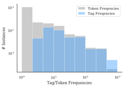
Effectiveness of Tags

The entire goal, in some sense, is for us to remove low-occurence, unimportant information from our data, and form concept conglomerates that allow more useful statistical inferences to be made. Tags from nestor-gui, as the next plot shows, have no instances of 1x-occurrence concepts, compared to several thousand in the raw-tokens (this is by design, of course). Additionally, high occurence concepts that might have had misspellings or synonyms drastically inprove their average occurence rate.

cts = (tex._model.transform(raw_text)>0.).astype(int).toarray().sum(axis=0)
# cts2 = (tex3._model.transform(replaced_text2)>0.).astype(int).toarray().sum(axis=0)

sns.distplot(cts,
#              np.concatenate((cts, cts2)),
             bins=np.logspace(0,3,10),
#              bins=np.linspace(0,1500,10),
             norm_hist=False,
             kde=False,
             label='Token Freqencies',
             hist_kws={'color':'grey'})
# cts
sns.distplot(tag_df[['I', 'P', 'S']].sum(),
             bins=np.logspace(0,3,10),
#              bins=np.linspace(0,1500,10),
             norm_hist=False,
             kde=False,
             label='Tag Freqencies',
             hist_kws={'hatch':'///', 'color':'dodgerblue'})

plt.yscale('log')
plt.xscale('log')
tag_df.sum().shape, cts.shape
plt.legend()
plt.xlabel('Tag/Token Frequencies')
plt.ylabel('# Instances')
sns.despine()
plt.savefig('toks_v_tags.png', dpi=300)

# tag-completeness of work-orders?
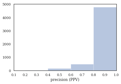
tag_pct, tag_comp, tag_empt = kex.get_tag_completeness(tag_df)

# with sns.axes_style('ticks') as style:
sns.distplot(tag_pct.dropna(),
             kde=False, bins=nbins,
             kde_kws={'cut':0})
plt.xlim(0.1, 1.0)
plt.xlabel('precision (PPV)')

Tag completeness: 0.94 +/- 0.13
Complete Docs: 4444, or 81.02%
Empty Docs: 48, or 0.88%

Text(0.5,0,'precision (PPV)')

Convergence over time, using nestor-gui

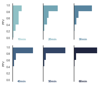
As part of the comparison study, an expert used nestor-gui for approximately 60min annotating 1-grams, followed by 20min focusing on 2-grams. Work was saved every 10 min, so we would like to see how the above plot was arrived at as the tokens were classified.

study_fname = Path('.')/'support'/'vocab_study_results.csv'
study_df = pd.read_csv(study_fname, index_col=0)
study_long = pd.melt(study_df, var_name="time", value_name='PPV').dropna()
study_long['time_val'] = study_long.time.str.replace('min','').astype(float)

sns.set(style="white", rc={"axes.facecolor": (0, 0, 0, 0)}, context='paper')
pal = sns.cubehelix_palette(6, rot=-.25, light=.7)
g = sns.FacetGrid(study_long, col="time", hue="time", aspect=.8, height=2, palette=pal, col_wrap=3)
g.map(sns.distplot, "PPV", kde=False, bins=nbins, vertical=True,
      hist_kws=dict(alpha=1., histtype='stepfilled', edgecolor='w', lw=2))
g.map(plt.axvline, x=0, lw=1.4, clip_on=False, color='k')

# Define and use a simple function to label the plot in axes coordinates
def label(x, color, label):
    ax = plt.gca()
    ax.text(.2, 0, label, fontweight="bold", color=color,
            ha="left", va="center", transform=ax.transAxes)
g.map(label, "PPV")

# Remove axes details that don't play well with overlap
g.set_titles("")
g.set( xticks=[], xlabel='')
g.set_axis_labels(y_var='PPV')
g.despine(bottom=True, left=True)
plt.tight_layout()

Survival Analysis

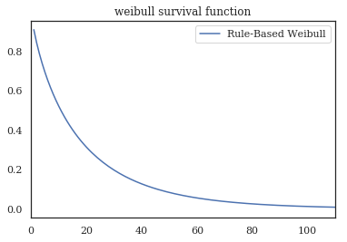
Rules-Based

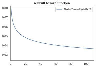
From Hodkeiwiz et al, a rule-based method was used to estimate failure times for SA. Let’s see their data:

df_clean = dat.load_excavators(cleaned=True)

df_clean['SuspSugg'] = pd.to_numeric(df_clean['SuspSugg'], errors='coerce')
df_clean.dropna(subset=['RunningTime', 'SuspSugg'], inplace=True)

df_clean.shape

(5288, 17)

df_clean.sort_values('BscStartDate').head(10)

	BscStartDate	Asset	OriginalShorttext	PMType	Cost	RunningTime	MajorSystem	Part	Action	Variant	FM	Location	Comments	FuncLocation	SuspSugg	Rule	Unnamed: 16
8	2001-07-19	B	REPLACE LIP	PM01	1251.52	7.0	Bucket	NaN	Replace	2V	NaN	NaN	NaN	Bucket	0.0	Rule_1_3_78_383_384	NaN
1820	2001-09-01	B	OIL LEAK L/H TRACK TENSIONER.	PM01	0.00	3.0	Hydraulic System	Track	Minor Maint	18	Leak	Left	NaN	Power Train - Transmission	0.0	Rule_1_3_52_289_347_425_500	NaN
1821	2001-09-04	B	BAD SOS METAL IN OIL	PM01	0.00	3.0	Hydraulic System	Slew Gearbox	NaN	NaN	Contamination	NaN	NaN	Sprocket/Drive Compartment Right	0.0	Rule_1_3_52_303_409	NaN
5253	2001-09-05	B	REPLACE AIRCONDITIONER BELTS	PM01	0.00	23.0	NaN	Air Conditioning	Replace	2V	NaN	NaN	NaN	Air Conditioning System	0.0	Rule_1_3_224_227_383_384	NaN
3701	2001-09-05	B	REPLACE CLAMPS ON CLAM PIPES	PM01	0.00	28.0	NaN	Mount	Replace	2V	NaN	NaN	NaN	Oil - Hydraulic	0.0	Rule_1_3_92_181_383_384	NaN
1167	2001-09-05	B	REPLACE RHS FAN BELT TENSIONER PULLEY	PM01	82.09	0.0	NaN	Fan	Minor Maint_Replace	2V	NaN	Right	NaN	+Cooling System	0.0	Rule_1_3_125_347_383_384_509	NaN
1168	2001-09-11	B	replace fan belt	PM01	0.00	6.0	NaN	Fan	Replace	2V	NaN	NaN	NaN	+Cooling System	0.0	Rule_1_3_125_383_384	NaN
644	2001-09-15	B	replace heads on lhs eng	PM01	0.00	33.0	Engine	NaN	Replace	2V	NaN	Left	NaN	Engine Left Cylinder Heads	0.0	Rule_1_3_25_383_384_499	NaN
4583	2001-09-26	B	REPAIR CABIN DOOR FALLING OFF.	PM01	0.00	27.0	NaN	Drivers Cabin	Repair	1	NaN	NaN	NaN	Operators Cabin	0.0	Rule_1_3_251_284_357	NaN
9	2001-10-01	B	rebuild lip #3	PM01	0.00	74.0	Bucket	NaN	Repair	5	NaN	NaN	NaN	Bucket Clam (Lip)	0.0	Rule_1_3_78_362	NaN

We once again turn to the library Lifelines as the work-horse for finding the Survival function.

from lifelines import WeibullFitter, ExponentialFitter, KaplanMeierFitter
mask = (df_clean.MajorSystem =='Bucket')
# mask=df_clean.index
def mask_to_ETclean(df_clean, mask, fill_null=1.):
    filter_df = df_clean.loc[mask]
    g = filter_df.sort_values('BscStartDate').groupby('Asset')
    T = g['BscStartDate'].transform(pd.Series.diff).dt.days
#     T.loc[(T<=0.)|(T.isna())] = fill_null
    E = (~filter_df['SuspSugg'].astype(bool)).astype(int)
    return T.loc[~((T<=0.)|(T.isna()))], E.loc[~((T<=0.)|(T.isna()))]

T, E = mask_to_ETclean(df_clean, mask)
wf = WeibullFitter()
wf.fit(T, E, label='Rule-Based Weibull')
print('{:.3f}'.format(wf.lambda_), '{:.3f}'.format(wf.rho_))
# wf.print_summary()
wf.hazard_.plot()
plt.title('weibull hazard function')
plt.xlim(0,110)

wf.survival_function_.plot()
plt.xlim(0,110)
plt.title('weibull survival function')
print(f'transform: β={wf.rho_:.2f}\tη={1/wf.lambda_:.2f}')
# wf._compute_standard_errors()
to_bounds = lambda row:'±'.join([f'{i:.2g}' for i in row])
wf.summary.iloc[:,:2].apply(to_bounds, 1)

0.060 0.833
transform: β=0.83       η=16.73

lambda_    0.06±0.0033
rho_        0.83±0.026
dtype: object

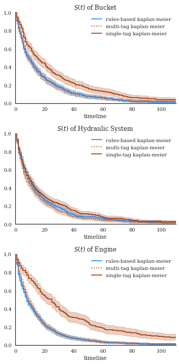
Tag Based Comparison

We estimate the occurence of failures with tag occurrences.

import math


def to_precision(x,p):
    """
    returns a string representation of x formatted with a precision of p

    Based on the webkit javascript implementation taken from here:
    https://code.google.com/p/webkit-mirror/source/browse/JavaScriptCore/kjs/number_object.cpp
    """

    x = float(x)

    if x == 0.:
        return "0." + "0"*(p-1)

    out = []

    if x < 0:
        out.append("-")
        x = -x

    e = int(math.log10(x))
    tens = math.pow(10, e - p + 1)
    n = math.floor(x/tens)

    if n < math.pow(10, p - 1):
        e = e -1
        tens = math.pow(10, e - p+1)
        n = math.floor(x / tens)

    if abs((n + 1.) * tens - x) <= abs(n * tens -x):
        n = n + 1

    if n >= math.pow(10,p):
        n = n / 10.
        e = e + 1

    m = "%.*g" % (p, n)

    if e < -2 or e >= p:
        out.append(m[0])
        if p > 1:
            out.append(".")
            out.extend(m[1:p])
        out.append('e')
        if e > 0:
            out.append("+")
        out.append(str(e))
    elif e == (p -1):
        out.append(m)
    elif e >= 0:
        out.append(m[:e+1])
        if e+1 < len(m):
            out.append(".")
            out.extend(m[e+1:])
    else:
        out.append("0.")
        out.extend(["0"]*-(e+1))
        out.append(m)

    return "".join(out)

def query_experiment(name, df, df_clean, rule, tag, multi_tag, prnt=False):

    def mask_to_ETclean(df_clean, mask, fill_null=1.):
        filter_df = df_clean.loc[mask]
        g = filter_df.sort_values('BscStartDate').groupby('Asset')
        T = g['BscStartDate'].transform(pd.Series.diff).dt.days
        E = (~filter_df['SuspSugg'].astype(bool)).astype(int)
        return T.loc[~((T<=0.)|(T.isna()))], E.loc[~((T<=0.)|(T.isna()))]

    def mask_to_ETraw(df_clean, mask, fill_null=1.):
        filter_df = df_clean.loc[mask]
        g = filter_df.sort_values('BscStartDate').groupby('Asset')
        T = g['BscStartDate'].transform(pd.Series.diff).dt.days
        T_defined = (T>0.)|T.notna()
        T = T[T_defined]
        # assume censored when parts replaced (changeout)
        E = (~(tag_df.S.changeout>0)).astype(int)[mask]
        E = E[T_defined]
        return T.loc[~((T<=0.)|(T.isna()))], E.loc[~((T<=0.)|(T.isna()))]

    experiment = {
        'rules-based': {
            'query': rule,
            'func': mask_to_ETclean,
            'mask': (df_clean.MajorSystem == rule),
            'data': df_clean
        },
        'single-tag': {
            'query': tag,
            'func': mask_to_ETraw,
            'mask': tag_df.I[tag].sum(axis=1)>0,
            'data': df
        },
        'multi-tag': {
            'query': multi_tag,
            'func': mask_to_ETraw,
            'mask': tag_df.I[multi_tag].sum(axis=1)>0,
            'data': df
        }
    }
    results = {
       ('query', 'text/tag'): [],
#        ('Weibull Params', r'$\lambda$'): [],
       ('Weibull Params', r'$\beta$'): [],
       ('Weibull Params', '$\eta$'): [],
       ('MTTF', 'Weib.'): [],
       ('MTTF', 'K-M'): []
       }
    idx = []

    for key, info in experiment.items():
        idx += [key]
        results[('query','text/tag')] += [info['query']]
        if prnt:
            print('{}: {}'.format(key, info['query']))
        info['T'], info['E'] = info['func'](info['data'], info['mask'])
        wf = WeibullFitter()
        wf.fit(info['T'], info['E'], label=f'{key} weibull')

        to_bounds = lambda row:'$\pm$'.join([to_precision(row[0],2),
                                             to_precision(row[1],1)])

        params = wf.summary.T.iloc[:2]
        params['eta_'] = [1/params.lambda_['coef'],  # err. propagation
                          (params.lambda_['se(coef)']/params.lambda_['coef']**2)]
        params = params.T.apply(to_bounds, 1)

        results[('Weibull Params', r'$\eta$')] += [params['eta_']]
        results[('Weibull Params', r'$\beta$')] += [params['rho_']]
        if prnt:
            print('\tWeibull Params:\n',
                  '\t\tη = {}\t'.format(params['eta_']),
                  'β = {}'.format(params['rho_']))

        kmf = KaplanMeierFitter()
        kmf.fit(info["T"], event_observed=info['E'], label=f'{key} kaplan-meier')
        results[('MTTF','Weib.')] += [to_precision(wf.median_,3)]
        results[('MTTF','K-M')] += [to_precision(kmf.median_,3)]
        if prnt:
            print(f'\tMTTF: \n\t\tWeib \t'+to_precision(wf.median_,3)+\
                   '\n\t\tKM \t'+to_precision(kmf.median_,3))
        info['kmf'] = kmf
        info['wf'] = wf
    return experiment, pd.DataFrame(results, index=pd.Index(idx, name=name))

bucket_exp, bucket_res = query_experiment('Bucket', df, df_clean,
                                          'Bucket',
                                          ['bucket'],
                                          ['bucket', 'tooth', 'lip', 'pin']);

tags = ['hyd', 'hose', 'pump', 'compressor']
hyd_exp, hyd_res = query_experiment('Hydraulic System', df, df_clean,
                                    'Hydraulic System',
                                    ['hyd'],
                                    tags)

eng_exp, eng_res = query_experiment('Engine', df, df_clean,
                                    'Engine',
                                    ['engine'],
                                    ['engine', 'filter', 'fan'])

frames = [bucket_res, hyd_res, eng_res]
res = pd.concat(frames, keys = [i.index.name for i in frames],
               names=['Major System', 'method'])
res

		query	Weibull Params		MTTF
		text/tag	$\beta$	$\eta$	Weib.	K-M
Major System	method
Bucket	rules-based	Bucket	0.83$\pm$0.03	17$\pm$0.9	10.8	9.00
	single-tag	[bucket]	0.83$\pm$0.03	27$\pm$2	17.1	15.0
	multi-tag	[bucket, tooth, lip, pin]	0.82$\pm$0.02	16$\pm$0.9	10.5	9.00
Hydraulic System	rules-based	Hydraulic System	0.86$\pm$0.02	14$\pm$0.6	9.07	8.00
	single-tag	[hyd]	0.89$\pm$0.04	36$\pm$3	24.1	25.0
	multi-tag	[hyd, hose, pump, compressor]	0.89$\pm$0.02	15$\pm$0.7	9.74	9.00
Engine	rules-based	Engine	0.81$\pm$0.02	17$\pm$1	10.8	9.00
	single-tag	[engine]	0.79$\pm$0.03	19$\pm$1	11.8	10.0
	multi-tag	[engine, filter, fan]	0.81$\pm$0.02	15$\pm$0.8	9.31	8.00

exp = [bucket_exp, eng_exp, hyd_exp]
f,axes = plt.subplots(nrows=3, figsize=(5,10))
for n, ax in enumerate(axes):
    exp[n]['rules-based']['kmf'].plot(ax=ax, color='dodgerblue')
    exp[n]['multi-tag']['kmf'].plot(ax=ax, color='xkcd:rust', ls=':')
    exp[n]['single-tag']['kmf'].plot(ax=ax, color='xkcd:rust')

    ax.set_xlim(0,110)
    ax.set_ylim(0,1)
    ax.set_title(r"$S(t)$"+f" of {res.index.levels[0][n]}")
    sns.despine()
plt.tight_layout()
f.savefig('bkt_KMsurvival.png')

/home/tbsexton/anaconda3/lib/python3.6/site-packages/matplotlib/cbook/__init__.py:2446: UserWarning: Saw kwargs ['c', 'color'] which are all aliases for 'color'.  Kept value from 'color'
  seen=seen, canon=canonical, used=seen[-1]))
/home/tbsexton/anaconda3/lib/python3.6/site-packages/matplotlib/cbook/__init__.py:2446: UserWarning: Saw kwargs ['c', 'color'] which are all aliases for 'color'.  Kept value from 'color'
  seen=seen, canon=canonical, used=seen[-1]))
/home/tbsexton/anaconda3/lib/python3.6/site-packages/matplotlib/cbook/__init__.py:2446: UserWarning: Saw kwargs ['c', 'color'] which are all aliases for 'color'.  Kept value from 'color'
  seen=seen, canon=canonical, used=seen[-1]))
/home/tbsexton/anaconda3/lib/python3.6/site-packages/matplotlib/cbook/__init__.py:2446: UserWarning: Saw kwargs ['c', 'color'] which are all aliases for 'color'.  Kept value from 'color'
  seen=seen, canon=canonical, used=seen[-1]))
/home/tbsexton/anaconda3/lib/python3.6/site-packages/matplotlib/cbook/__init__.py:2446: UserWarning: Saw kwargs ['c', 'color'] which are all aliases for 'color'.  Kept value from 'color'
  seen=seen, canon=canonical, used=seen[-1]))
/home/tbsexton/anaconda3/lib/python3.6/site-packages/matplotlib/cbook/__init__.py:2446: UserWarning: Saw kwargs ['c', 'color'] which are all aliases for 'color'.  Kept value from 'color'
  seen=seen, canon=canonical, used=seen[-1]))
/home/tbsexton/anaconda3/lib/python3.6/site-packages/matplotlib/cbook/__init__.py:2446: UserWarning: Saw kwargs ['c', 'color'] which are all aliases for 'color'.  Kept value from 'color'
  seen=seen, canon=canonical, used=seen[-1]))
/home/tbsexton/anaconda3/lib/python3.6/site-packages/matplotlib/cbook/__init__.py:2446: UserWarning: Saw kwargs ['c', 'color'] which are all aliases for 'color'.  Kept value from 'color'
  seen=seen, canon=canonical, used=seen[-1]))
/home/tbsexton/anaconda3/lib/python3.6/site-packages/matplotlib/cbook/__init__.py:2446: UserWarning: Saw kwargs ['c', 'color'] which are all aliases for 'color'.  Kept value from 'color'
  seen=seen, canon=canonical, used=seen[-1]))

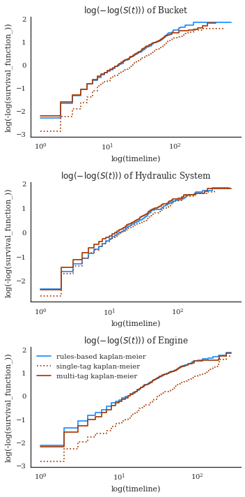
This next one give you an idea of the differences better. using a log-transform. the tags under-estimate death rates a little in the 80-130 day range, probably because there’s a failure mode not captured by the [bucket, lip, tooth] tags (because it’s rare).

f,axes = plt.subplots(nrows=3, figsize=(5,10))
for n, ax in enumerate(axes):
    exp[n]['rules-based']['kmf'].plot_loglogs(ax=ax, c='dodgerblue')
    exp[n]['single-tag']['kmf'].plot_loglogs(ax=ax, c='xkcd:rust', ls=':')
    exp[n]['multi-tag']['kmf'].plot_loglogs(ax=ax, c='xkcd:rust')
    if n != 2:
        ax.legend_.remove()
#     ax.set_xlim(0,110)
#     ax.set_ylim(0,1)
    ax.set_title(r"$\log(-\log(S(t)))$"+f" of {res.index.levels[0][n]}")
    sns.despine()
plt.tight_layout()
f.savefig('bkt_logKMsurvival.png', dpi=300)
# kmf.plot_loglogs()