[1]:
from pathlib import Path
import numpy as np
import pandas as pd
import seaborn as sns
import matplotlib.pyplot as plt
%matplotlib inline
[2]:
def set_style():
    # This sets reasonable defaults for font size for a figure that will go in a paper
    sns.set_context("paper")
    # Set the font to be serif, rather than sans
    sns.set(font='serif')
    # Make the background white, and specify the specific font family
    sns.set_style("white", {
        "font.family": "serif",
        "font.serif": ["Times", "Palatino", "serif"]
    })
set_style()
HVAC Maintenance Case Study
Import Data
[3]:
import nestor.keyword as kex
data_dir = Path('../..')/'data'/'hvac_data'
df = pd.read_csv(data_dir/'hvac_data.csv')
# really important things we know, a priori
special_replace={'action taken': '',
                 ' -': '; ',
                 '- ': '; ',
                 'too hot': 'too_hot',
                 'to hot': 'too_hot',
                 'too cold': 'too_cold',
                 'to cold': 'too_cold'}

nlp_select = kex.NLPSelect(columns = ['DESCRIPTION', 'LONG_DESCRIPTION'], special_replace=special_replace)
raw_text = nlp_select.transform(df)
/home/tbsexton/anaconda3/envs/nestor-dev/lib/python3.6/site-packages/IPython/core/interactiveshell.py:3020: DtypeWarning: Columns (29,30,40,106,172,196,217,227) have mixed types. Specify dtype option on import or set low_memory=False.
  interactivity=interactivity, compiler=compiler, result=result)
Build Vocab
[4]:
tex = kex.TokenExtractor()
toks = tex.fit_transform(raw_text)
print(tex.vocab_)
['room' 'poc' 'stat' ... 'llines' 'pictures' 'logged']
[5]:
vocab_fname = data_dir/'vocab.csv'
# vocab_fname = data_dir/'mine_vocab_app.csv'

# vocab = tex.annotation_assistant(filename = vocab_fname)
vocab = kex.generate_vocabulary_df(tex, init = vocab_fname)
intialized successfully!
Extract Keywords
[6]:
tag_df = kex.tag_extractor(tex, raw_text, vocab_df=vocab)
tags_read = kex._get_readable_tag_df(tag_df)
intialized successfully!
[7]:
tags_read.head(5)
[7]:
| I | NA | P | S | U | X | |
|---|---|---|---|---|---|---|
| 0 | pm, order, site, aml, charge | complete | ||||
| 1 | time | pm, cover, order, aml, charge, charged | need | |||
| 2 | point_of_contact, thermostat | ed | replace, adjust, reset, repair | freeze | ||
| 3 | point_of_contact, thermostat | ed | adjust, reset, repair, restart | freeze | ||
| 4 | thermostat | adjust, reset, repair | freeze |
[8]:
# vocab = pd.read_csv(data_dir/'app_vocab_mike.csv', index_col=0)
# how many instances of each keyword class are there?
print('named entities: ')
print('I\tItem\nP\tProblem\nS\tSolution\nR\tRedundant')
print('U\tUnknown\nX\tStop Word')
print('total tokens: ', vocab.NE.notna().sum())
print('total tags: ', vocab.groupby("NE").nunique().alias.sum())
vocab.groupby("NE").nunique()
named entities:
I       Item
P       Problem
S       Solution
R       Redundant
U       Unknown
X       Stop Word
total tokens:  5000
total tags:  86
[8]:
| NE | alias | notes | score | |
|---|---|---|---|---|
| NE | ||||
| 1 | 1 | 1 | 4650 | |
| I | 1 | 45 | 5 | 204 |
| P | 1 | 7 | 2 | 26 |
| S | 1 | 16 | 3 | 70 |
| U | 1 | 14 | 8 | 26 |
| X | 1 | 3 | 2 | 6 |
[9]:
# tag-completeness of work-orders?
tag_pct, tag_comp, tag_empt = kex.get_tag_completeness(tag_df)
nbins = int(np.percentile(tag_df.sum(axis=1), 90))
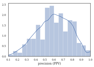
print(f'Docs have at most {nbins} tokens (90th percentile)')
sns.distplot(tag_pct.dropna(), bins=nbins, kde_kws={'cut':0})
plt.xlim(0.1, 1.0)
plt.xlabel('precision (PPV)')
Tag completeness: 0.60 +/- 0.19
Complete Docs: 254, or 1.50%
Empty Docs: 126, or 0.74%
Docs have at most 20 tokens (90th percentile)
[9]:
Text(0.5, 0, 'precision (PPV)')
Measuring Machine Performance
[10]:
import nestor.tagplots as tagplt
samp = ['air_conditioning_unit','fan', 'valve', 'leak', 'too_hot', 'too_cold']
cond = (tag_df.P.alarm==1)
sample_tag = tag_df.loc[:,(slice(None), samp)]
sample_tag.columns = sample_tag.columns.droplevel(0)

idx_col = pd.DatetimeIndex(df.REPORTDATE)
sample_tag = sample_tag.set_index(idx_col[:])
sample_tag = sample_tag[ sample_tag.index.year.isin([2009, 2010, 2016])]


tagplt.tagcalendarplot(sample_tag,
                  how='sum', fig_kws={'figsize':(13,8)});
plt.suptitle('Tag Occurence')
[10]:
Text(0.5, 0.98, 'Tag Occurence')
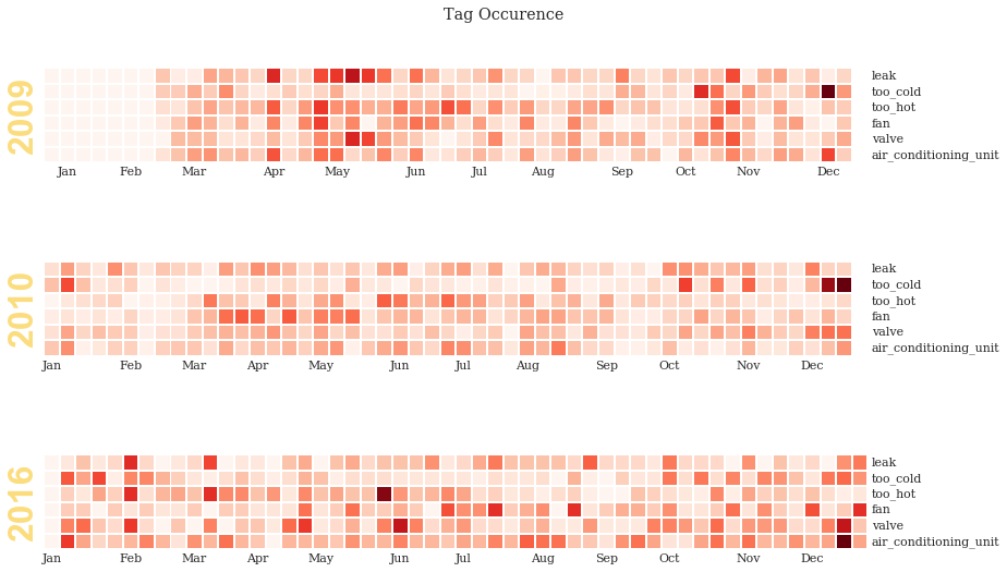
Monthly “too-hot” and “too-cold” requests, over time
[18]:
import holoviews as hv
import geoviews as gv
hv.extension('bokeh')


[146]:
%%output size=200
temp_curve_spec = {
#     'Spread':{'plot':{'width':300, 'height':80},
#               'style':dict(line_color=None, alpha=.4, color=hv.Cycle(['#fe420f', '#06b1c4']))},
    'Curve':{'plot':{'width':300, 'height':80}},
    'Curve.TooHot':{'style':dict(color='#fe420f')},
    'Curve.TooCold':{'style':dict(color='#06b1c4')},
    'NdOverlay': {'plot':dict(title='Requests')}
}
#     'Scatter':{'style':dict( size=5, color=hv.Cycle(['#fe420f', '#06b1c4']))}

# hv.Cycle(['#fe420f', '#06b1c4'])

samp = ['too_cold', 'too_hot']
sample_tag = tag_df.loc[:,(slice(None), samp)]
sample_tag.columns = sample_tag.columns.droplevel(0)

sample_tag = sample_tag.set_index(idx_col).sort_index()

# resamp = '30D'
resamp = '1W'
meas = sample_tag[pd.datetime(2009,9,1):pd.datetime(2012,3,1)].resample(resamp).sum()
meas['date'] = meas.index
# roll = sample_tag.rolling('10D').mean()
# mean = sample_tag.rolling('1D').mean().resample(resamp).sum()
# err =  sample_tag.rolling('1D').std().resample(resamp).sum()

# temp_curves = hv.Overlay([
# #     hv.Spread((mean.index, mean.too_hot, err.too_hot)),
# #     hv.Spread((mean.index, mean.too_cold, err.too_cold)),
#     hv.Curve((meas.index, meas.too_hot)),
#     hv.Curve((meas.index, meas.too_cold)),
# #     hv.Scatter((meas.index, meas.too_hot), label='too_hot'),
# #     hv.Scatter((meas.index, meas.too_cold), label='too_cold')
# ])

# table = hv.Table(meas, ['too_hot', 'too_cold'], 'date')
temp_curves = hv.NdOverlay({
    'too_cold':hv.Curve(meas,'date', 'too_cold', group='Requests', name='TooCold'),
    'too_hot':hv.Curve(meas, 'date','too_hot', group='Requests', name='TooHot'),
}).opts(temp_curve_spec)
# temp_curves.select().opts(temp_curve_spec)#*hv.VLine(times[5])
# hv.Curve(table)

# temp_curves.select(date=(pd.datetime(2010,1,1),pd.datetime(2012,1,1)))
# temp_curves.select(too_hot=(meas.too_hot.quantile(.25),meas.too_hot.quantile(.75)))

# meas[pd.datetime(2010,1,1):pd.datetime(2012,1,1)]
temp_curves
[146]:
[147]:
pd.datetime(2010, 1, 1)
[147]:
datetime.datetime(2010, 1, 1, 0, 0)
[148]:
import geopandas as gpd
nist_df = gpd.read_file(str(data_dir/'nist_map.geojson')).set_index('bldg', drop=False)
nist_df.index = nist_df.index.astype(str)
samp = ['too_cold', 'too_hot']
sample_tag = tag_df.loc[:,(slice(None), samp)]
sample_tag.columns = sample_tag.columns.droplevel(0)

bldg_col = df.LOCATION.str.split('-').str[0].astype('category')
sample_tag = pd.concat([sample_tag, bldg_col], axis=1)
sample_tag = sample_tag.set_index(idx_col).sort_index()
sample_tag.rename({'LOCATION':'bldg'}, axis='columns', inplace=True)

times = sample_tag.loc['2010-1-1':'2012-1-1'].resample('1QS').sum().index
# pd.concat([sample_tag.loc[times[0]:times[1]].groupby('bldg').sum(), nist_df], axis=1).dropna()

def get_bldg_temp(n):
    data = gpd.GeoDataFrame(pd.concat([sample_tag.loc[times[n]:times[n+1]].groupby('bldg').sum(),
                      nist_df],
                     axis=1).dropna())
    data['Temperature Index'] = np.tanh((data['too_cold'].sum()+data['too_hot'].sum())/20)*\
    (data['too_cold'] - data['too_hot'])
    return data
# np.tanh((data['too_cold'].sum()+data['too_hot'].sum())/20)*\
get_bldg_temp(1).head()
[148]:
| too_hot | too_cold | bldg | geometry | Temperature Index | |
|---|---|---|---|---|---|
| bldg | |||||
| 101 | 34 | 14 | 101.0 | POLYGON ((-77.2163987159729 39.13512015465694,... | -20.0 |
| 202 | 4 | 2 | 202.0 | POLYGON ((-77.22025036811827 39.13047428646352... | -2.0 |
| 203 | 0 | 0 | 203.0 | POLYGON ((-77.22077608108521 39.13020796677279... | 0.0 |
| 205 | 0 | 0 | 205.0 | POLYGON ((-77.21850156784058 39.1223198699503,... | 0.0 |
| 215 | 0 | 0 | 215.0 | POLYGON ((-77.21671521663666 39.1316623096919,... | 0.0 |
[149]:
from bokeh.palettes import Viridis10, Category10_6, RdBu10
from bokeh.models.mappers import LinearColorMapper
RdBu10.reverse()
padding = dict(x=(-77.223, -77.214), y=(39.13, 39.14))
extents = (-77.223, 39.129, -77.214, 39.1385)

bldg_dict, vlines = {}, {}
for n, time in enumerate(times[:-1]):
    mapped = gv.Polygons(get_bldg_temp(n),
                         vdims=['Temperature Index', 'bldg', 'too_hot', 'too_cold'],
                         extents = extents)
    mapped = mapped.redim.range(**padding)
    vlines[time] = hv.VLine(time).opts(style={'color':'black'})
    bldg_dict[time] = mapped

text = hv.Overlay([gv.Text(i.centroid.x-.0002,
                           i.centroid.y-.00015,
                           str(name)) for name,i in get_bldg_temp(0).geometry.iteritems()])
[150]:
%%output size=200 filename='nist_hvac_map'
%%opts Polygons [height=350 width=300, tools=['hover'] colorbar=False ] (cmap='RdBu')
%%opts VLine (alpha=.5)

import warnings
warnings.simplefilter(action='ignore', category=FutureWarning)

(hv.HoloMap(bldg_dict, 'Time')*text +\
 hv.HoloMap(vlines, 'Time')*\
 temp_curves.opts(temp_curve_spec)).cols(1)
# hv.Bounds()
[150]:
[ ]: